Equations

Home

What follows is a brief explanation of the equations that were used to generate the output of this calculator. For a more thorough explanation of the derivation and application of these equations, you are encouraged to explore some of the many excellent microscopy resources, such as:

Nikon MicroscopyU
Zeiss Microscopy Online Campus
The Handbook of Biological Confocal Microscopy

Equations Used

The lateral resolution of a microscope, defined as the minimum distance between two distinguishable objects and measured as the radius of the first dark ring around the central disk of the Airy diffraction image, is given by the Abbe Equation:

r_{lat} = 0.61* \frac{\lambda_{em}}{NA}

where λ_em is the emission wavelength and NA is the numerical aperture of the objective.

The axial resolution, defined as the distance from the center of the 3D diffraction pattern to the first axial minimum (in object space dimensions), is given by:

r_{ax} = 2 * \frac{\lambda_{em} * n}{NA^2}

where n is the refractive index of the media. It should be noted here that, for spinning disk microscopy, the observed axial resolution will probably be far worse than that predicted by the preceding formula. Issues arising from "cross-talk" of light from neighboring pinholes will lower the effective axial resolution. The Handbook of Biological Confocal Microscopy gives the following equation for axial resolution near the focal plane of slit and point scan confocal microscopes with very small pinhole/slit dimensions

dz = K * \frac{\lambda}{n[1-\sqrt{1-(NA^2/n)^2}]}

where K is a scalar correction factor that equals 0.67 for pinhole disks. In the future, I hope to incorporate this equation into the calculator as well.

In confocal microscopy, the term "confocality" is often used to as an indication of how well out of focus light is eliminated from the final image. This is largely determined by how well the physical size of the pinhole is matched to the lateral resolution of the optical system. First, one needs to know the size of the pinhole in the sample plane, known as the "back-projected" pinhole, which can be calculated as

r_{pinhole_{BP}} = \frac{r_{pinhole}}{M_{obj} * M_{csu}}

where r_pinhole is the radius of the physical pinhole, and M_obj and M_csu are the magnifications of the objective lens and the CSU relay (if present), respectively.

Confocality can then be represented as "Airy Units", which is simply the ratio of the back-projected pinhole radius to the radius of the Airy Disk (given by the equation for lateral resolution above):

AU = \frac{r_{pinhole_{BP}}}{r_{lateral}}

In order to fully capture all of the information provided by the resolution of the optical system, the Nyquist criterion states that the sampling frequency should be 2.4X higher than the highest spatial frequency in the data. In this case, the highest possible spatial frequency is the given by a diffraction limited point source of light: in other words, the lateral resolution. Thus, in order to fully represent the optical data in our digitized image, the size of the camera pixel when projected onto the object plane (the back-projected pixel) should be at least 2.4 times less than the size of the Airy radius. In order to calculate the back-projected pixel size, we use the equation:

pix_{BP} = \frac{pix_{cam}*Binning}{M_{tot}}

where pix_cam is the physical size of a pixel on the camera chip, Binning is the binning settings on the camera, and M_tot is the total magnification in the optical train between the sample and the camera chip, including the objective and any other optical relays present.

The sampling frequency, or sampling "rate", then can be represented as the ratio of the radius of the Airy Disk, r_lat, to the size of the back-projected pixel.

f_{s} = \frac{r_{lat}}{pix_{BP}}

One additional consideration in microscopy is the field of view (FOV). For the purpose of this calculator, we are only interested in the field of view captured by the camera. When considering the camera, field of view becomes a conditional measurement, depending on whether the entire camera chip is used or not. The following equation describes the relation of the microscope field aperture to the camera chip for the width (w) and height (h) of the camera chip. When ChipUsed is greater than 1, then the entire chip has been used in that dimension (width or heigh).

ChipUsed_{w/h} = \frac{Aperture_{w/h}* M_{cam}}{Chip_{w/h}}

where Aperture_w/h refers to the dimension of the microscope field aperture, or the Confocal Aperture, in the case of spinning disks (which is usually the more limiting dimension when calculating field of view with spinning disks), and Chip_w/h refers to the width or height of the physical camera chip.

If the illuminated sample does not fill the camera chip (in other words: if the camera is able to image the entire illuminated sample) then the field of view is equal to the illuminated sample. Which is measured as such:

IlluminatedSample_{w/h} = \frac{Aperture_{w/h}}{M_{obj} * M_{csu}}

On the other hand, if an appropriate camera relay is used such that the entire camera chip is illuminated, then the calculation for field of view in either the width or height dimension becomes simply

FOV_{w/h} = \frac{Chip_{w/h}}{M_{tot}}

The "show chip" display on the calculator is designed to help clarify the measurements of FOV.

Back

Tutorial

The Airy Disk

The graphic in the calculator is a representation of the airy disk: the image that a diffraction limited point source (such as a single molecule of GFP) projects onto the camera due to the finite aperture of the objective lens. For the purpose of the calculator, the graphic is a simply computer generated representation of a true airy pattern, and the outer rings have been slightly amplified for clarity.

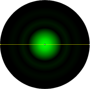
A line scan across the center of the image reveals the (approximated) airy disk profile.

The radius r_Airy of the first dark ring around the central disk of the Airy diffraction image depends on wavelength and the NA of the objective, and defines the theoretical limit to lateral resolution.

r_{airy} = 0.61* \frac{\lambda_{em}}{NA}

Nyquist Sampling

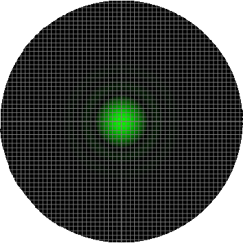
In order to properly sample the resolution available in the digitization of a microscopic image, the Nyquist criteria states that the smallest feature in the image (the airy disk) should be at least 4 pixels wide. Therefore, in our image, the Airy radius should sampled by at least 2 pixels. The grid on the calculator graphic represents the size of the back-project pixel (the camera pixel as it would appear in the image plane after). Alternatively, the image can be thought of as the size of airy disk projected on the camera chip itself. The image below represents an image of a single EGFP fluorophore, imaged with a 20X / 0.5 NA objective onto a camera with a 6.45 µm pixel size (such as the Clara). Here, the radius of the Airy disk is slightly smaller than two pixels on the camera, corresponding to a sampling rate of 1.93 pixels / r_airy. Hence, we are slightly undersampling the resolution available here.

The following image represents the image of the Airy disk produced by an EGFP molecule imaged through a 100X / 1.4 NA objective onto a camera with a 3.63 µm pixel size, such as the Orca-Flash2.8. Here it can be seen that our sampling rate is over 6 pixels / r_airy and we are drastically oversampling the resolution available. In this scenario, it would be appropriate to either bin the camera, or to use a camera relay of less than 1X mag.

Confocality & Airy Units

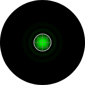
In confocal microscopy, the pinhole is present to prevent light originating from anywhere but the plane of focus from reaching the detector. The "optimal" size of the pinhole is about 1 "Airy Unit" (AU), which corresponding to the size of the central circle of the airy disk pattern. In this calculator, a pinhole size of 1 AU means that the radius of the backprojected pinhole (the pinhole projected onto the sample) is the same size as the airy radius, r_airy. The image below represents an EGFP molecule imaged through a 60X / 1.4 NA objective onto a camera with a 6.45 µm pixel size. The white circle represents the size of the pinhole. On the Yokogawa CSU-X1, the pinhole is fixed at a 50 µm diameter. As the image shows, with this configuration, the pinhole size is 1.9 AU, nearly two times larger than the size of the airy disk.

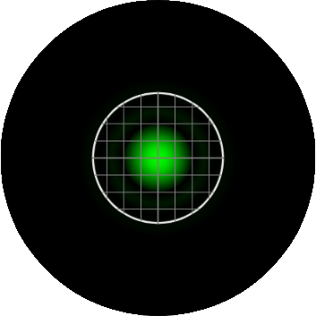
The Yokogawa CSU-W1 head has the option of a second disk with a pinhole size of 25 µm. If we take the configuration from the image above, and swap out the 50µm disk for the 25µm disk, the backprojected pinhole gets smaller and is now more closely matched to the size of the inner circle of the airy disk (0.9 AU), as displayed in the image below.

Spinning Disk vs Laser Scanning Confocals

Although it has many benefits with regards to photon efficiency and speed, one of the major disadvantages of a spinning disk confocal microscope is the inability to change the size of the pinhole. While newer systems such as the Yokogawa CSU-W1 allow one to change the physical disk and the Spectral Borealis modification to the CSU-X1 grants some flexibility with the size of the "effective" (backprojected) pinhole, we are still largely limited when it comes to the size of the pinhole in spinning disk microscopy. Similarly, though CCD and sCMOS chips have significantly better quantum efficiency than the PMTs used in laser scanning confocals, they do not grant the user the same sort of flexibility with regards to Nyquist sampling that the "arbitrary" pixel size of the PMT does. Thus, we must take advantage of differing combinations of objectives and optical relays to optimize the sampling rate in our digital image. We will usually not be able to find a setting on spinning disk microscope that allows us to image with both "optimal" confocality of 1 AU and a sampling rate of 2 pixels per airy radius. However, this calculator is designed to help with the optimization process.

iScopeCalc

My Scopes